
Machine Learning for Backend Developers in the Age of Large Models

Preface
From the emergence of the Transformer architecture in 2017 to the arrival of GPT in 2022, people have increasingly recognized the importance of large models, to the point that every year seems to be proclaimed the inaugural year of LLMs. As we gradually enter the AI era, I feel both deeply anxious, worried that large models might replace me, and excited by the prospect of doing more with LMs.
But what can I do with LLMs? And what do I need to understand?
Before the age of large models, backend developers could generally start building software once they had mastered a programming language such as Java, Go, or JavaScript, along with architectural knowledge of MySQL and Redis. In the AI era—or, more precisely, the age of large models—knowing only conventional programming languages is clearly no longer enough.
LLM engineering can be summed up in one sentence: using all kinds of prompts to call LLMs, accompanied by engineering capabilities such as MCP and RAG. If you want to quickly embed LM capabilities into a business scenario, it is essentially the same as being a CRUD developer in the old days: simply call the open APIs provided by large-model vendors.
Yet merely calling a model’s API is like looking at the moon reflected in water or flowers reflected in a mirror: you never truly see the essence or the whole system. In my view, for backend developers who want to become part of the AI era, the first step should not be calling LLM-related APIs. It should be understanding the concepts and principles behind traditional artificial intelligence and machine learning. What exactly is the relationship between ML and DL? How did architectures such as CNNs, RNNs, and Transformers evolve? Without this basic knowledge, it is like programming without understanding operating systems or computer networks—you can complete basic development tasks, but cannot go further and glimpse the wonders of the computing world.
So I spent some time organizing my understanding of artificial intelligence and machine learning around a number of common questions.
Your AI and My AI Seem to Be Different
In recent years, with the rise of large models, everything has become AI. In the narrow sense, AI means artificial intelligence, and the people primarily responsible for implementing it are called “algorithm engineers” (often jokingly called parameter tuners). In the age of large models, many people use large models as a synonym for AI. Luo Yonghao, for example, has consistently argued that the true AI era did not arrive until 2023. So what are the relationships and differences among artificial intelligence, machine learning, deep learning, and large models?
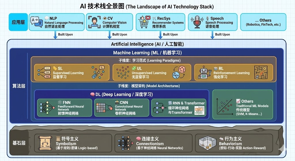
According to Hung-yi Lee’s framework, we generally regard Artificial Intelligence (AI) as the ultimate goal and Machine Learning (ML) as the primary means of achieving it. Computer Vision (CV), Natural Language Processing (NLP), and similar fields are specific applications.
From a layperson’s perspective, ML is an umbrella term whose core logic is to “train models with data so that computers learn patterns independently and complete specific tasks.” Among the technical branches of ML, Deep Learning (DL) is currently the most central and mainstream direction. Deep learning uses “deep neural networks” as its core architecture, with multiple layers containing many neurons that learn. In increasing order of complexity, neural networks include basic Feedforward Neural Networks (FNNs), Recurrent Neural Networks (RNNs) for sequential data, and Convolutional Neural Networks (CNNs) for spatial data. Google’s Transformer architecture restructured the sequential processing principles used by RNNs and CNNs. By adopting a Self-Attention mechanism, it addressed sequence dependency problems, allowing a model both to perceive relationships among tokens and to train in parallel.
As for Large Models (LMs), “large” refers not only to their number of parameters but also to the volume of data required for training. It was the Transformer that made scaling models to this size possible. One of the earliest branches of large models was the Large Language Model (LLM), which originated in NLP and is suited to conventional NLP tasks such as text generation. With the development of multimodal LMs, however, large models are no longer confined to NLP; in pursuit of the broader goal of AI, they have reached into every kind of application.
What Can Machine Learning Do?
At the application level, ML-based LLMs can generate text from text, images from text, text from images, and more. At their root, however, all application tasks ultimately return to two categories: “regression” and “classification.”
Regression is similar to y=kx+b: different inputs produce different values. Regression tasks are commonly used for prediction, such as weather forecasts, house prices, and stock trends. Classification builds on regression and uses an activation or classification function to divide results into categories, such as positive and negative. Classification tasks are commonly used for labeling.
The recommendation component in search, recommendation, and advertising systems is a classification task. As is widely known, although a large model generates text according to predicted probabilities, it is essentially predicting the next word (Token) from a vocabulary of, say, 50,000 words. Large models therefore perform classification tasks.
What Exactly Is a Model?
With the widespread adoption of large models, almost everyone has heard the word “model.” But what exactly is one?
At a high level, a model is a black box. You provide input to the model, computations take place inside it, and it ultimately returns an output.
Looking at the open-source model repository on Hugging Face, a model looks like this:
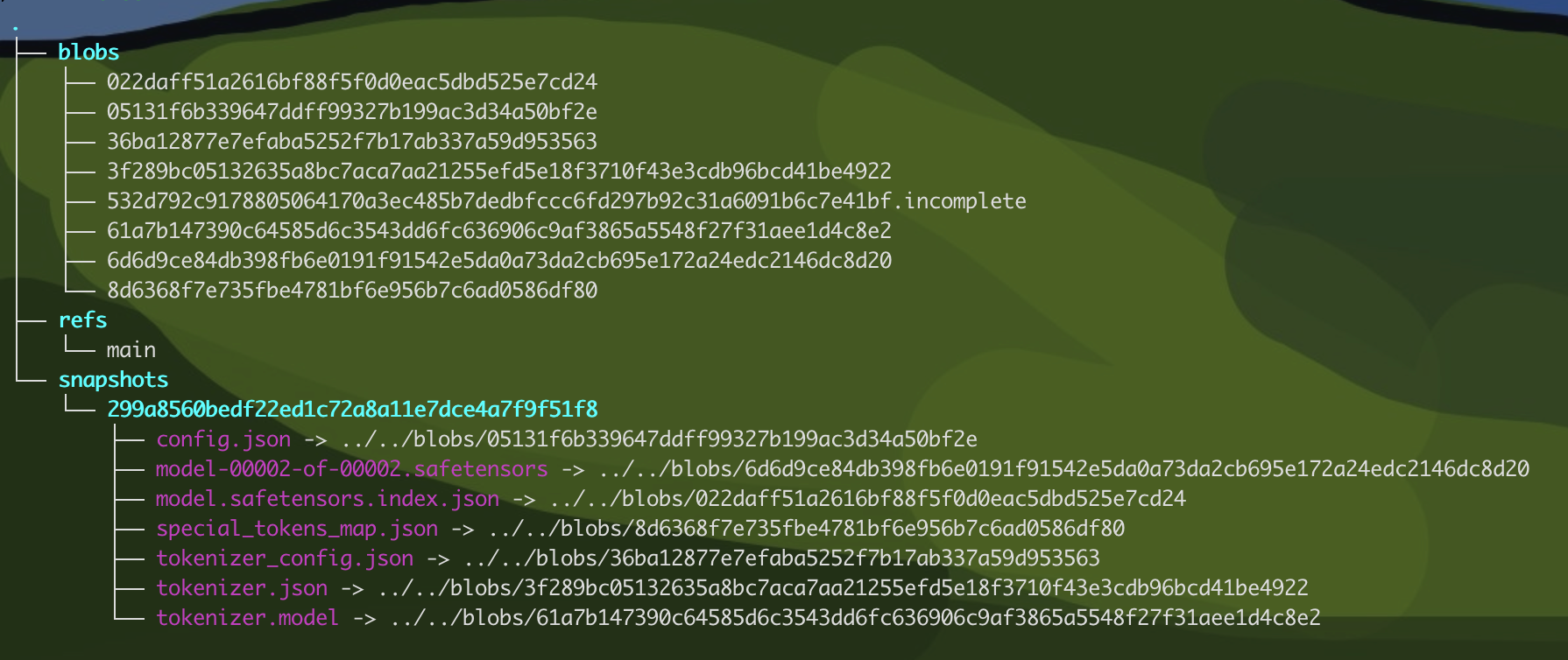
Inside a model is a collection of parameters (weights). What we call the model’s thinking process is essentially a series of vector operations—mainly matrix multiplication—performed together with the input tokens. In the age of large models, we can narrow our focus and think of the model as a neural network composed of many neurons. So what exactly is a neuron?
Neurons and Neural Networks
Neurons
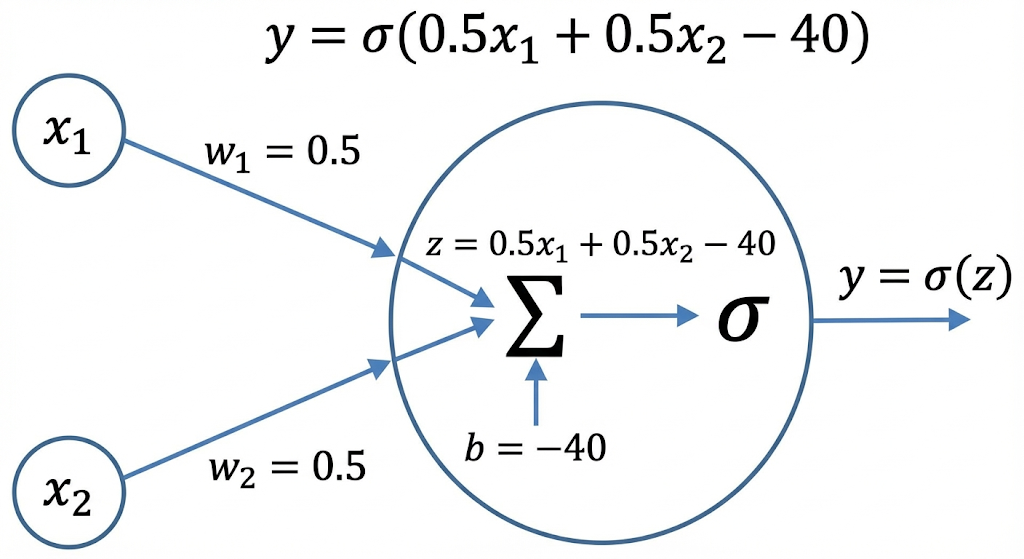
A neuron can be understood simply as a computational unit. Given an input x, the neuron might compute wx+b, and its calculated output can be y. The difference is that x is not a single variable of the kind encountered in high-school mathematics, but a one-dimensional vector made up of n variables related to the input:
\(y = \sigma(w_1 x_1 + w_2 x_2 + b)\), that is:
\(y = \sigma([w_1, w_2] \cdot \begin{bmatrix} x_1 \\ x_2 \end{bmatrix} + b)\)
In the expression above, \(x_1\) and \(x_2\) are input features. For example, in a weather forecasting model, \(x_1\) might be humidity and \(x_2\) might be temperature. \(w_1\) and \(w_2\) are the variables’ weights, also known as “parameters.” Training means continually adjusting the values of \(w\) (and other parameters) so that the output \(y\) approaches the true value and the loss becomes lower. \(b\) is the bias—or, in simpler terms, the intercept—which can increase or decrease the computed value. The symbol outside the parentheses is sigma (\(\sigma\)), representing the activation function. Common activation functions include Sigmoid (\(\sigma(x) \in (0,1)\)) and ReLU (\(relu(x) = max(0,x)\)). Activation functions control the output and make the result nonlinear.
A visual representation of a neuron is shown below:
A simple neuron can be expressed in Python as follows:
1 | import torch |
Suppose the trained parameters are \(w_1=0.5, w_2=0.5, b=-40\), giving \(y = \sigma(0.5 x_1 + 0.5 x_2 - 40)\). We obtain the prediction trend shown below:
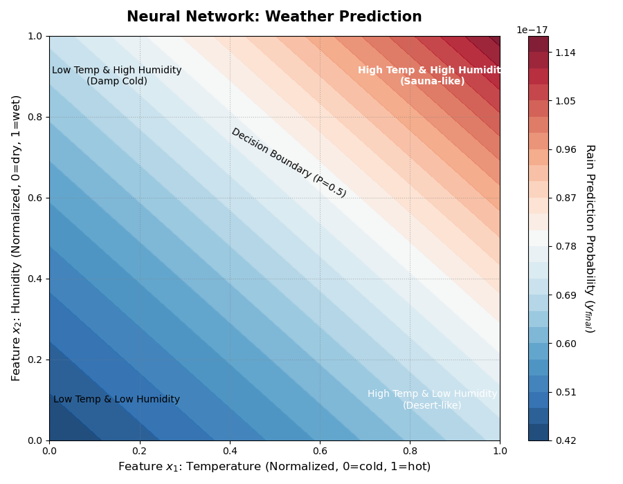
From the diagram, we would conclude that higher temperature and higher humidity make rain more likely. Let us examine the cases:
- Case A (sauna-like weather): \(0.9 \times 0.5 + 0.9 \times 0.5 = 0.9\) (predicts rain, correct ✅)
- Case B (desert): \(0.9 \times 0.5 + 0.0 \times 0.5 = 0.45\) (predicts no rain, correct ✅)
- Case C (extreme heat and dryness): suppose the temperature is exceptionally high, \(x_1=2.0\):
- \(2.0 \times 0.5 + 0.0 \times 0.5 = 1.0\) (predicts rain, incorrect ❌)
We find that even if the trained w and b are optimal, the result is necessarily linear. Weather forecasting, however, is not a linear prediction problem. We therefore need to try other tools to solve it.
Fully Connected Neural Networks
As we can see, a simple neuron can only perform linear regression. The real world is complex, so we need to connect multiple neurons together to perform more complex tasks.
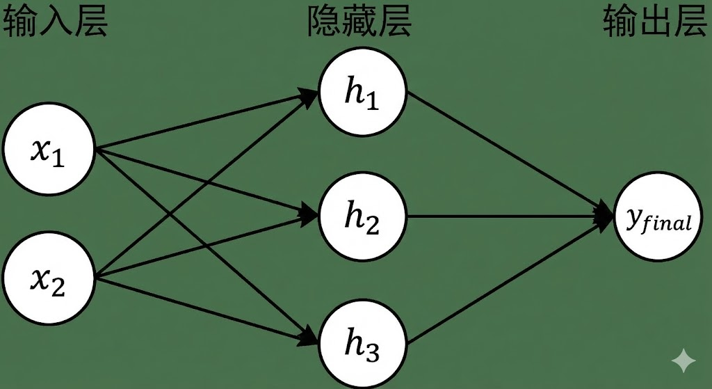
The weather forecasting example tells us that forecasting weather is not a linear prediction problem. The weather features are related, yet a single neuron cannot capture those relationships. From an engineering perspective, when in doubt, add an intermediate layer. Since temperature and humidity are related, we can associate them to form multiple intermediate features, then use those intermediate features to produce the final result, as shown below:
Converted into simple mathematical formulas, this becomes:
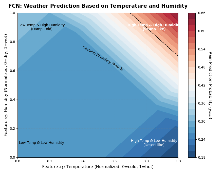
Because the formulas above connect \(x_1, x_2\) as completely as possible, we call this network a Fully Connected Network (FCN), which forms the foundation of modern deep learning. Applying this FCN to our humidity and temperature example, let \(h_1\) represent sauna-like conditions, \(h_2\) cold and humid conditions, and \(h_3\) hot and dry conditions. Suppose training produces the following result:
We obtain the prediction diagram below. As you can see, after adding the intermediate layer, the model no longer predicts rain under “hot and dry” conditions.
Returning to the mathematical formulas, if there are many features and multiple layers of neurons, the preceding notation becomes far too complicated. Using the spatial transformation properties of matrix multiplication—rotation, scaling, and distortion—we can rewrite the hidden layer as follows:
,
The final output is therefore:
\(y_{final} = \sigma( \underbrace{\begin{bmatrix} v_1 & v_2 & v_3 \end{bmatrix}}_{W_2} \cdot \underbrace{\begin{bmatrix} h_1 \\ h_2 \\ h_3 \end{bmatrix}}_{h} + b_4 )\).
When training in code, however, we want to parallelize as much of the work as possible, which introduces the concept of batching. Instead of calculating one feature sample at a time, we group samples into a batch and calculate several at once, using the following formula:
,
That is:
\(h_{\text{单层输出}} = xW^T + b\)
In code:
1 | class SimpleFCN(nn.Module): |
CNNs and RNNs
With FCNs, we can theoretically use enough data to train for any result we want. But because FCNs are fully connected, they have three major drawbacks:
- Parameter redundancy and high computational cost: By default, every neuron connects to every neuron in the previous layer, causing the number of parameters to rise sharply. When the input dimensionality is high, as in high-resolution images, or the network has many layers, this can cause a parameter explosion that exhausts the computer’s memory.
- Local features are ignored: Because every FCN computation must consider all inputs, it has no concept of “spatial locality.” It cannot behave like the human eye, first focusing on local features such as lines and textures and then combining them into a whole. Instead, it processes all information in one undifferentiated gulp.
- No awareness of “order”: In an FCN, all input features are parallel, so the network cannot perceive which came “before” and which came “after.” For example, when we feed a Sentence into an FCN as Input, the FCN cannot effectively capture temporal dependencies among Tokens, making it difficult to understand contextual meaning.
CNN
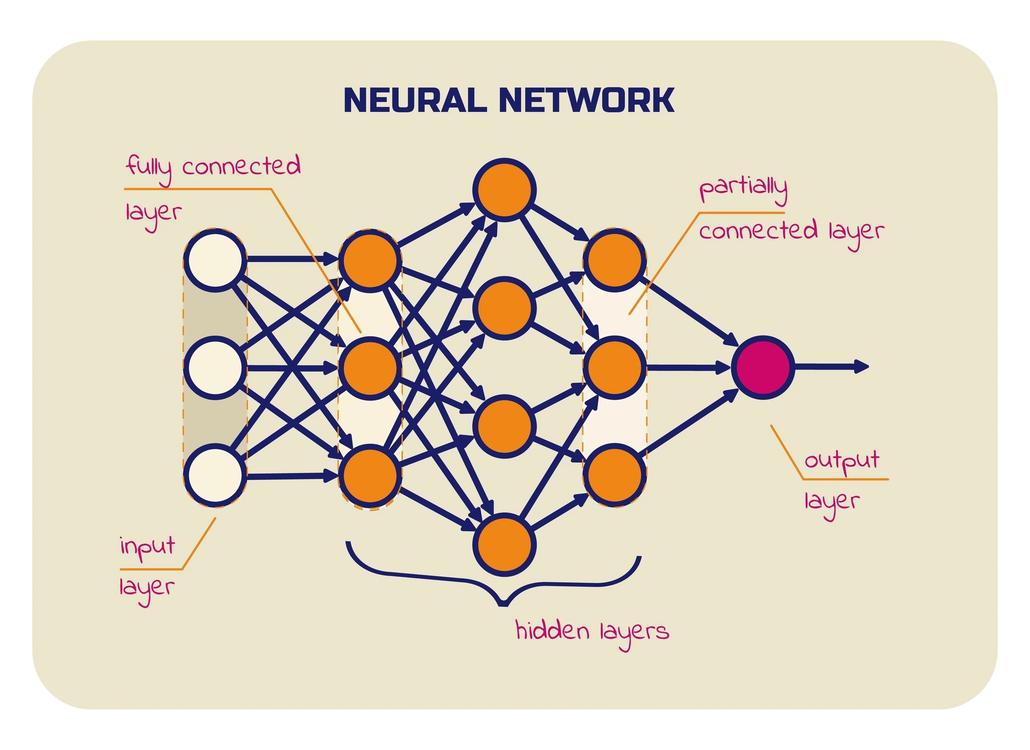
A CNN, or Convolutional Neural Network, centers on a convolutional layer. Unlike an FCN, this layer does not connect every neuron to all parameters; it connects them “selectively.”
Suppose we have a 33-pixel image. If we use an FCN to recognize it, we must flatten the 33 pixels into nine parameters and perform fully connected linear operations on them. A single neuron can be expressed mathematically as follows:
,
\(h = \sigma(w_{1} x_1 + w_{2} x_2 + ... + w_n x_n + ... + w_9 x_9 + b) \\\)
Flattening almost completely removes positional and spatial information from the parameters. Using an FCN therefore causes not only a parameter explosion, but also a reduction in recognition accuracy.
For images, preserving positional information means we cannot flatten the input pixels. We must consider the relationships among pixel values. At the same time, to avoid computing every pixel each time, we need a window so that each neuron calculates only the values inside that window. If the window is 2x2, it can be represented as follows:
This Kernel is the convolution kernel. The neuron can now be expressed as:
\(h = \sigma(w_{1,1} x_1 + w_{1,2} x_2 + w_{2,1} x_4 + w_{2,2} x_5 + b) \\\)
As we can see, a convolution-kernel neuron has two characteristics: first, it does not process all parameters; second, it can precisely perceive position-related information.
The essence of a convolution kernel is that it focuses on local features instead of all features. We can think of a convolution kernel as a local feature detector. Suppose \(K_h\) has 22 parameters and is specifically responsible for recognizing “vertical lines.” \(K_h\) slides up, down, left, and right through every 22 block of pixels to find blocks that might contain a “vertical line.”
An image has more than one feature, so we use multiple convolution kernels (\(K_1,..., K_n\)), each representing a different feature. Some kernels may recognize lines, others colors, and so on.
A simple CNN is shown below:
1 | import torch |
RNN
FCNs transform user-provided features into more general features, while CNNs go further by handling certain relationships among features. Neither FCNs nor CNNs, however, address relationships among features across time. Consider this scenario:
While performing machine translation, we try to translate “Book a hotel” and “I like book” into Chinese.
If we directly train an FCN on the sentences above, each token in “Book a hotel” must be used as a training parameter. That is certainly feasible, but once the sentence to translate changes to “I like book,” the original FCN becomes completely unusable because its input parameters have a fixed shape. An FCN alone is therefore wholly inadequate when the input varies.
Since training the complete sentence is impractical, we must split it into words and train on them separately. In other words, the input cannot be fed all at once as it is in an FCN; it must be fed incrementally. Yet because “book” has different meanings in different sentences, when we input the current word we must also retain some preceding words and provide them to the model as input.
Can we therefore design a network that 1) dynamically perceives input tokens and 2) perceives not only the current token but previous tokens as well? That is precisely an RNN (Recurrent Neural Network).
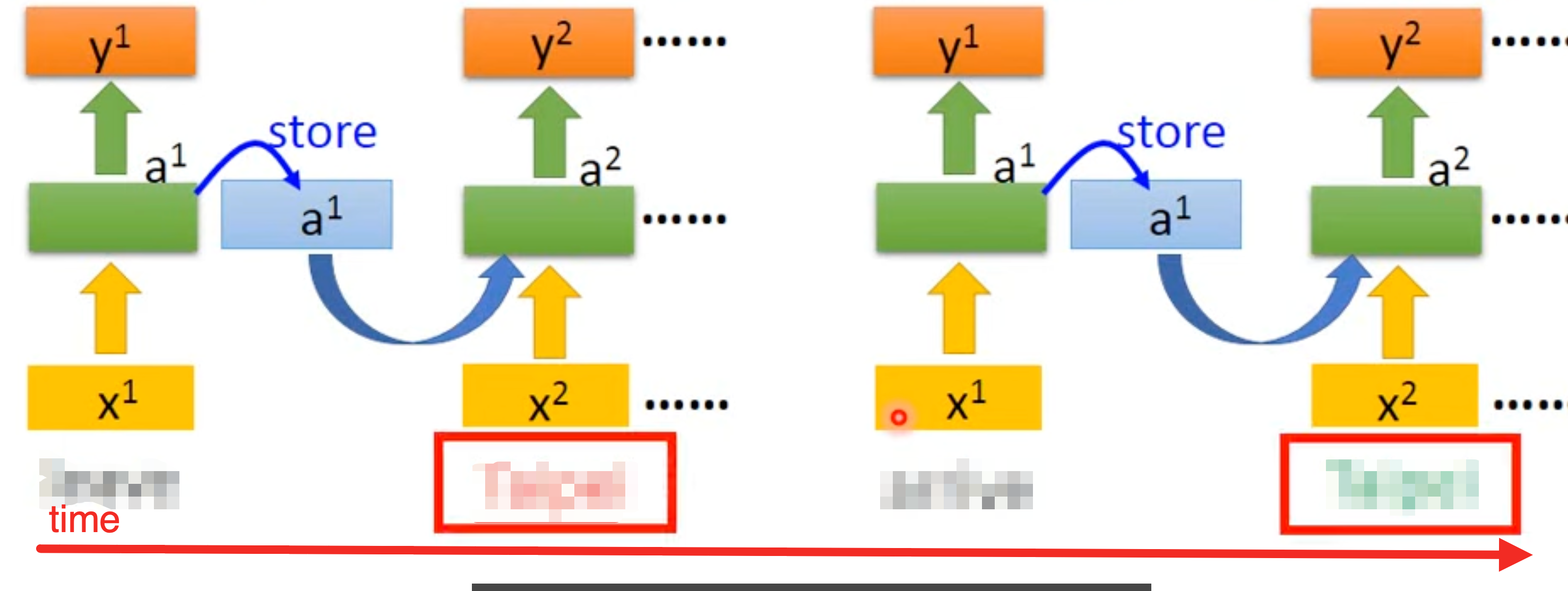
At its core, an RNN adds a recurrent mechanism to an FCN, enabling it to perceive the preceding output. Its mathematical expression is:
The formula shows that the essence of an RNN is to feed the result calculated from the previous input into the next computation as another input. The Python code is as follows:
1 | import torch |
There is one important detail: if the weight is 0.9, then as the number of propagation layers grows, \(0.9^{n}\) approaches 0. This means an RNN cannot remember very long inputs; overly long inputs cause it to “forget,” a phenomenon known as the vanishing-gradient problem. This led to the development of LSTM, which uses an Input Gate, Output Gate, and Forget Gate to decide when to store memories and to control the model’s forgetting more precisely.
What Exactly Are a Model’s Parameters?
From the FCN, CNN, and RNN models above, we can see that a model is essentially \(y = \sigma(kx+b)\). Its so-called parameters are therefore \(k\) (the weight, or w) and b (the bias). A real model simply has n$ values of x and m values of y. As n and m (as well as the neurons in the intermediate hidden layers) increase, there are more weights and biases, and the trained model becomes more “intelligent.” This is the popular industry understanding of the “large” in “large model.”
Training a model means using various mathematical methods to calculate the most effective weights and biases. Take GPT-3 as an example: it has 175B (175 billion) parameters, meaning that the w and b values across all its neurons add up to 175 billion.
TODO-Hyperparameters.
How Does a Model Understand Natural Language?
So far, we have learned how a model performs inference: given an input x, where x is a tensor, it applies a series of formula-based operations and produces an output. This raises a question. Whether we use an FCN, RNN, or CNN, the model can only perform floating-point operations, so its input must be a group of numbers. That works well enough for ordinary mathematical predictions. But for today’s flourishing field of natural language processing, how do we turn natural language into numbers that a model can understand?
One-Hot
The simplest approach is to use a Boolean-array mapping. Given a Boolean array of fixed length, we identify different tokens by marking different indexes as true. Suppose your vocabulary contains only five words: ["我", "爱", "学习", "AI", "猫"]. The word “学习” is represented as [0, 0, 1, 0, 0].
One-hot encoding has two fatal problems that prevent it from being used in LLMs:
- Sparsity and the curse of dimensionality: A real vocabulary contains tens or even hundreds of thousands of words. Each word becomes a vector of length 50,000 containing 49,999 zeros. This wastes enormous computational resources.
- Lack of semantic relationships (Semantic Meaning): In One-Hot space, the distance between every pair of words is identical. The distance between “cat” and “dog” is the same as the distance between “cat” and “refrigerator.” The model cannot know that “cat” and “dog” are similar.
Embedding
Embedding lets us compress one-hot’s high-dimensional sparse vectors into low-dimensional dense vectors. For example, we can map “cat” to a 512-dimensional vector:
\(\text{Embedding(cat)} = [0.21, -0.54, 0.03, ..., 0.99]\)
In this new vector space, words with similar meanings are closer together geometrically. For example, we can approximately say:
\("国王" - "男人" + "女人" \approx "女王"\)
How do we obtain a set of dense vectors capable of retaining relationships among words? The method is straightforward: perform unsupervised training and transformation with an FCN. Here is an example:
Calculate the five-dimensional one-hot vectors for “机器 学习 改变 了 世界” and convert them into three-dimensional dense vectors.
- Define one-hot vectors for the five tokens. For example, the one-hot vector for 学习 is \(x = [0, 1, 0, 0, 0]\).
- Define a linear regression network in which W has a 5x3 structure, then substitute the x for “学习” as follows:
- Next, calculate the dot product of \(h\) and another transposed matrix, \(W_{out}\):
\(z = \sigma(h \cdot W_{out} = h \cdot [u_0, u_1, u_2, u_3, u_4])\)
- This gives the probabilities relating “学习” to each token in the original sentence. Suppose the calculated dot-product result is:
\(\hat{z} = [0.05, \quad 0.02, \quad \mathbf{0.80}, \quad 0.01, \quad 0.12]\)
This means there is an 80% probability that “改变” follows “学习,” but we want that probability to be 100%. We therefore need to update the values in W through backpropagation. After multiple rounds of training, \(W_{input}\) becomes our final embedding vectors.
How Does a Machine Learn?
We have repeatedly emphasized that we need to train models so they can learn independently. How, then, does a model learn?
Before examining the learning process in depth, we need to understand two terms: Forward Propagation and Backpropagation.
Forward Propagation
Forward propagation is quite simple to explain. The FCN, CNN, and RNN computations described above are all forward propagation, expressed as:
\(y_{pred} = \text{Model}(x)\)
During forward propagation, the parameters (Weight and bias) are known and given. In fact, when we use GPT or Gemini, the process by which the model produces an answer is forward propagation.
Backpropagation
Backpropagation is the reverse of forward propagation. Given \(y_{pred},y_{true},LearningRate\), it is the process of calculating the parameters \(Weight, Bais\).
To define exactly how far apart \(y_{pred}\) and \(y_{true}\) are, we generally use a Loss Function. This is the Loss commonly discussed when training models: the larger the Loss, the worse the model’s result. A common loss function is Mean Squared Error:
\(Loss = (y_{pred} - y_{true})^2\)
To reduce Loss, we use backpropagation together with the Gradient Descent algorithm, calculating new weights through differentiation according to this formula:
\(W_{new} = W_{old} - \text{learning\_rate} \times \text{Gradient}\)
Learning_rate is the step size, which determines how much the weights change in each training iteration. You can search for details on how the Gradient is calculated; I will not cover them here. An example of backpropagation follows:
1 | import torch |
Why Do GPUs Rule the World?
Before exploring this question, let us distinguish CPUs from GPUs:
- CPU: A CPU has a small number of powerful cores—our typical servers, for example, may have eight cores. It handles complex computations and logical branches, adding caches, control units, and other components to its computational units.
- GPU: A GPU has many simpler cores—even an ordinary one may have 4,096. Each core has limited capabilities and can perform only simple arithmetic rather than complex logic.
From model inference and training, we know that both forward propagation and backpropagation involve vast numbers of vector-product operations and differentiations. At heart, these are simple floating-point operations. Such operations basically do not interfere with one another, so they are naturally suited to “parallel” computation, making them an excellent fit for GPU architecture.
For example, multiplying two 1000x1000 matrices requires roughly one billion multiply-add operations. Even with eight parallel threads, an eight-thread CPU will take a long time to process them. A GPU has many more cores, so it is naturally much faster.
References
- Hung-yi Lee’s materials: YouTube (in Chinese), Bilibili (in Chinese)
- Gemini
- Datawhale: https://github.com/datawhalechina